Introduction: Why This Matters
Understanding wireless communication isn’t just about knowing that “data travels through the air.” It’s about understanding how a sequence of bits becomes electromagnetic waves, how those waves propagate through space, and how a receiver reconstructs the original data from noisy RF signals.
This article documents my journey building a complete LoRa communication system using two HackRF One software-defined radios. But more importantly, it explains why each component exists, how the signal processing chain works, and what actually happens when you press “transmit.”
If you’ve ever wondered how your phone talks to a cell tower, how Wi-Fi works, or how IoT devices communicate over kilometers this is your starting point.
Part 1: Understanding the Basics
What Problem Are We Solving?
The fundamental challenge in wireless communication is this:
How do we reliably send digital data (1s and 0s) through an analog medium (radio waves) in the presence of noise, interference, and hardware imperfections?
This isn’t trivial. Consider what needs to happen:
- Encoding: Convert your message (“HELLO”) into a format suitable for transmission
- Modulation: Map those bits onto a radio wave
- Propagation: The wave travels through space, picking up noise
- Reception: Capture the weak, noisy signal
- Demodulation: Extract the bits from the received wave
- Decoding: Reconstruct the original message
Each step introduces potential failure points. Let’s understand them one by one.
Part 2: The Hardware Foundation
What is a Software Defined Radio?
Traditional radios use dedicated hardware circuits for modulation, filtering, and demodulation. A Software Defined Radio (SDR) moves these functions into software, giving you complete control over every aspect of the communication system.
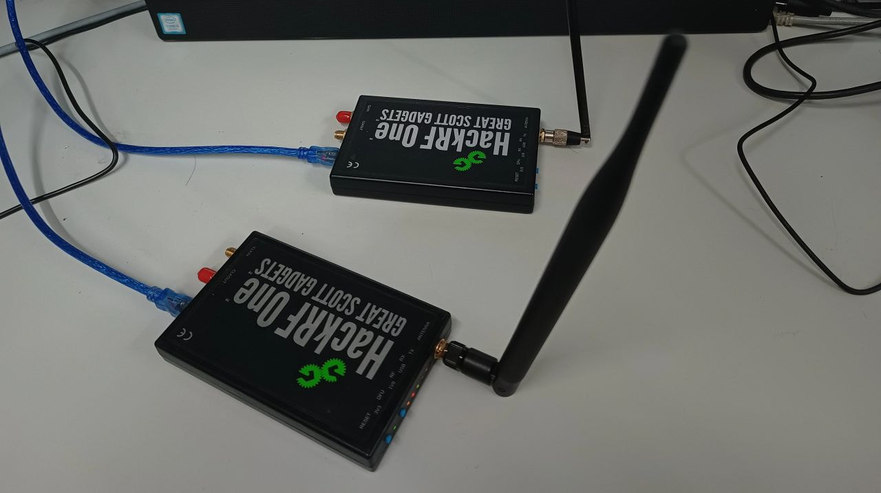
The HackRF One operates from 1 MHz to 6 GHz and can both transmit and receive. It connects via USB and streams I/Q samples (more on this later) to your computer, where GNU Radio processes them.
Why two HackRFs?
One acts as the transmitter, converting digital data into RF signals. The other acts as the receiver, capturing those signals and converting them back to data. This separation lets us debug each side independently.
Operating Frequency: 865.4025 MHz
I chose this frequency because:
- It falls within India’s 865-867 MHz ISM (Industrial, Scientific, Medical) band
- It’s license-free for low-power operation
- It’s designated for LoRa/LoRaWAN applications
- It has relatively low ambient interference compared to 2.4 GHz
Part 3: Starting Simple - FM Reception
Before attempting digital communication, I needed to verify the hardware worked. The simplest test? Build an FM radio receiver.
Why FM First?
FM (Frequency Modulation) is analog and well-understood. If you can’t receive FM stations, your hardware setup has issues. No point debugging digital protocols if basic RF reception doesn’t work.
I tuned to 93.5 MHz and 91.1 MHz both strong local stations. Audio came through clearly, confirming:
- Antenna connections were solid
- HackRF was receiving correctly
- GNU Radio flowgraph execution worked
- Sample rates and frequency tuning were accurate
This baseline test is critical. Always verify your hardware with a known-good signal before debugging custom protocols.
Part 4: Understanding Digital Modulation
From Bits to Waves: The Core Challenge
Digital data consists of discrete values (0s and 1s). Radio waves are continuous analog signals. Modulation is the bridge between these two worlds.
The basic idea:
- Choose a carrier wave (a pure sine wave at your transmission frequency)
- Vary some property of that wave to represent your data
- The receiver detects these variations and reconstructs your bits
Common Modulation Schemes
Frequency Shift Keying (FSK)
- Bit 0 → transmit at frequency f1
- Bit 1 → transmit at frequency f2
- Simple but susceptible to frequency drift
Binary Phase Shift Keying (BPSK)
- Bit 0 → phase = 0°
- Bit 1 → phase = 180°
- More robust than FSK but requires phase synchronization
Why I Started Here
FSK and BPSK are conceptually simple, making them good learning tools. I expected to build a working system quickly.
I was wrong.
Part 5: My First Failures - FSK and BPSK
The Transmitter Side: Deceptively Easy
Building the transmitter was straightforward:
Message "HELLO"
→ Convert to bytes: [72, 69, 76, 76, 79]
→ Convert to bits: [01001000, 01000101, ...]
→ Map bits to symbols (FSK frequencies or BPSK phases)
→ Generate I/Q samples
→ Send to HackRF
The HackRF transmitted. I could see the signal on a spectrum analyzer. Energy was radiating at 865 MHz exactly as expected.
Success, right? Not even close.
The Receiver Side: Where Everything Broke
The receiver needs to:
- Tune to the correct frequency
- Capture I/Q samples
- Detect the presence of a signal (not just noise)
- Synchronize timing (when does one bit end and the next begin?)
- Demodulate (extract bit values from the carrier)
- Reconstruct bytes (group bits correctly)
- Convert back to text
Every single one of these steps failed at some point.
Problem 1: Symbol Timing
The transmitter sends bits at a specific rate say, 10,000 bits per second. The receiver must sample at exactly the right moments.
Why is this hard?
- The transmitter and receiver have separate clocks
- Clocks drift slightly (even “precise” oscillators)
- By the time you’ve received 1000 bits, timing might be off by several samples
- You’re now reading between bits instead of at bit centers
Solution: Timing recovery algorithms. The receiver must continuously adjust its sampling clock to stay aligned with the transmitter.
Problem 2: Frame Synchronization
Even if you’re sampling at the right rate, where does the packet start?
Radio is a continuous stream. The receiver sees:
...noise...noise...signal...signal...noise...
How do you detect the boundary between “noise before the packet” and “actual packet data”?
Solution: Preambles. Transmit a known pattern before your data. The receiver correlates against this pattern to detect packet start.
Problem 3: Carrier Frequency Offset
Even if both devices are set to 865.4025 MHz, they won’t be exactly there.
- HackRF has ~20 ppm frequency error
- At 865 MHz, 20 ppm = 17.3 kHz offset
- Your signal appears shifted in frequency
- Demodulation fails because you’re looking in the wrong place
Solution: Carrier frequency offset estimation and correction. The receiver must detect the actual frequency and adjust.
Problem 4: Phase Ambiguity (BPSK specific)
In BPSK, you encode bits as 0° or 180° phase shifts. But the receiver doesn’t know the absolute phase only relative changes.
If you start with the phase inverted, every bit is flipped:
Transmitted: 01001000
Received:    10110111
Solution: Differential encoding (encode data as phase changes, not absolute phases) or use a known preamble to resolve ambiguity.
Why I Couldn’t Get FSK/BPSK Working
Each of these problems requires careful implementation. I was fighting:
- Timing drift
- Frequency offset
- Phase ambiguity
- Noise
- Sample rate mismatches
Simultaneously.
After weeks of debugging, I had partial success sometimes the receiver would decode correctly, but reliability was terrible. I needed a more robust approach.
Part 6: Enter LoRa - A Different Philosophy
What Makes LoRa Different?
LoRa (Long Range) doesn’t use FSK or BPSK. It uses Chirp Spread Spectrum (CSS).
What’s a chirp?
A chirp is a signal whose frequency increases (up-chirp) or decreases (down-chirp) linearly over time.
Imagine a sine wave that starts at 865.000 MHz and sweeps up to 865.250 MHz over 1 millisecond. That’s an up-chirp.
Why Chirps?
Chirps have unique properties:
- Time-Frequency Duality: A chirp’s frequency encodes time information
- Noise Immunity: Spread over wide bandwidth, making narrow-band interference less effective
- Doppler Resilience: Chirps remain recognizable even if frequency-shifted
- Processing Gain: Spreading signal energy improves SNR after demodulation
How LoRa Encodes Data
Instead of encoding bits as “frequency A or B” (FSK) or “phase 0 or 180” (BPSK), LoRa encodes bits as the starting frequency of a chirp.
With spreading factor SF=11:
- Each symbol represents 11 bits
- There are 2^11 = 2048 possible symbols
- Each symbol is a chirp starting at a different frequency
Example:
- Symbol 0 → chirp starts at the lowest frequency in the band
- Symbol 1 → chirp starts slightly higher
- Symbol 2047 → chirp starts at the highest frequency
The receiver performs an FFT on each received chirp, finds the peak frequency, and recovers the symbol.
Key LoRa Parameters
Bandwidth (BW): 250 kHz
- The range of frequencies the chirp sweeps across
- Wider = faster data rate but more susceptible to interference
Spreading Factor (SF): 11
- Number of bits per symbol
- Higher SF = longer chirps = longer range but slower data rate
- SF=11 means each symbol takes 2^11 / BW = 2048 / 250000 = 8.192 ms
Coding Rate (CR): 4/5
- Forward error correction ratio
- For every 4 data bits, transmit 5 bits total (1 bit redundancy)
- Helps correct transmission errors
Part 7: The LoRa Transmitter - Block by Block
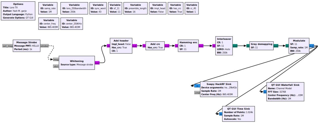
Let’s walk through every block in the transmitter chain and understand why it exists.
Block 1: Message Source
blocks.message_strobe(pmt.intern("HELLO"), 1000)
This generates the message “HELLO” every 1000 milliseconds.
Why PMT (Polymorphic Type)?
GNU Radio uses PMTs to pass messages between blocks. pmt.intern("HELLO") converts the string into a PMT that other blocks can process.
Block 2: Whitening
Purpose: Randomize the data to prevent long sequences of identical bits.
Why does this matter?
If you transmit “AAAAAAA…” (01000001 repeated), you get:
01000001010000010100000101000001...
This creates patterns in the RF spectrum that can interfere with synchronization and demodulation. Whitening applies a pseudo-random XOR sequence to break up these patterns.
Implementation:
XOR original data with a known pseudo-random sequence
Receiver XORs with the same sequence to recover original data
Block 3: Header Generation
Purpose: Add metadata about the packet.
The header contains:
- Payload length: How many bytes of actual data follow
- Coding rate: Which error correction rate is used
- CRC present: Whether a checksum is included
The receiver needs this information to correctly decode the payload.
Block 4: CRC (Cyclic Redundancy Check)
Purpose: Detect transmission errors.
A CRC is a mathematical checksum. The transmitter calculates it over the payload and appends it. The receiver recalculates the CRC and compares—if they don’t match, the packet is corrupted.
How it works:
- Treat your data as a large binary number
- Divide by a generator polynomial (a specific binary number)
- The remainder is your CRC
- Receiver performs the same division—if remainder is zero, data is valid
Block 5: Hamming Encoding (Forward Error Correction)
Purpose: Add redundancy so the receiver can correct errors without retransmission.
With CR=4/5, for every 4 data bits, you send 5 bits total. The extra bit provides error correction.
How it works:
Hamming codes add parity bits at specific positions. If a single bit flips during transmission, the receiver can identify which bit and correct it.
Example (simplified):
Original:  1011
Encoded:   10111
           ↑ parity bit inserted
If received as 10101 (bit 3 flipped), the receiver calculates:
Parity checks indicate bit 3 is wrong
Flip it back: 10101 → 10111
Decode: 1011 ✓
Block 6: Interleaving
Purpose: Spread burst errors across multiple symbols.
Radio interference often comes in bursts—a fraction of a second where multiple bits are corrupted. Without interleaving:
Data:     [1 0 1 1] [0 1 0 0] [1 1 0 1]
Burst error:         ↑↑↑↑↑↑↑↑
Result:   [1 0 1 1] [X X X X] [1 1 0 1]
          ✓ correct   ✗ lost    ✓ correct
An entire symbol is destroyed, overwhelming error correction.
With interleaving, bits from different symbols are mixed:
Symbol 1: bits 0, 3, 6, 9...
Symbol 2: bits 1, 4, 7, 10...
Symbol 3: bits 2, 5, 8, 11...
Now a burst error affects one bit per symbol:
Burst affects bits 4,5,6,7
→ One bit error in symbol 1
→ One bit error in symbol 2
→ One bit error in symbol 3
Hamming coding can correct single-bit errors, so all three symbols are recovered.
Block 7: Gray Mapping
Purpose: Convert bits to symbol numbers such that adjacent symbols differ by only one bit.
Why?
If demodulation makes an error and picks a symbol adjacent to the correct one, only one bit is wrong instead of multiple bits.
Example:
Binary:  00, 01, 10, 11
Gray:    00, 01, 11, 10
Notice 01 and 11 differ by one bit, not two.
Block 8: Modulation
Purpose: Generate the actual chirp waveforms.
For each symbol (0 to 2047), generate a chirp that starts at the corresponding frequency offset.
Parameters:
- SF=11 → 2048 chips per symbol
- BW=250 kHz → chirp sweeps 250 kHz
- Each chirp lasts 2048 / 250000 = 8.192 ms
The modulator outputs I/Q samples representing these chirps.
Block 9: HackRF Sink
Purpose: Convert I/Q samples to RF and transmit.
The HackRF’s digital-to-analog converter (DAC) generates the voltage waveforms, the mixer upconverts to 865 MHz, the amplifier boosts power, and the antenna radiates.
Configuration:
- Sample rate: 1 MSPS
- Center frequency: 865.4025 MHz
- TX gain: 35 dB (VGA gain)
- Amplifier: Enabled
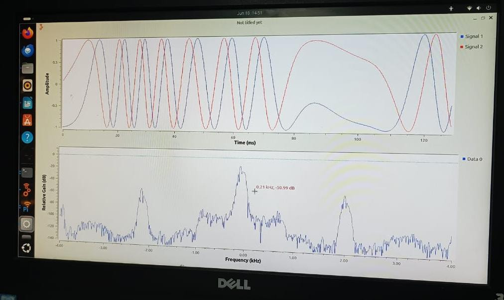
Part 8: Visualizing the Transmission
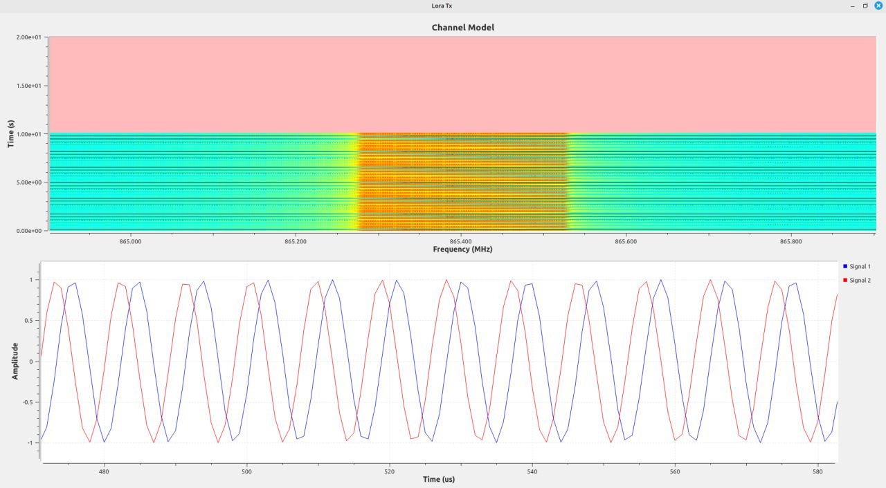
The top plot (waterfall) shows frequency on the horizontal axis, time on the vertical axis, and signal strength as color intensity.
You can see:
- The preamble: repeated up-chirps
- The sync word: inverted chirps
- The payload: chirps starting at different frequencies encoding data
The bottom plot shows the time-domain signal—the complex waveform being transmitted.
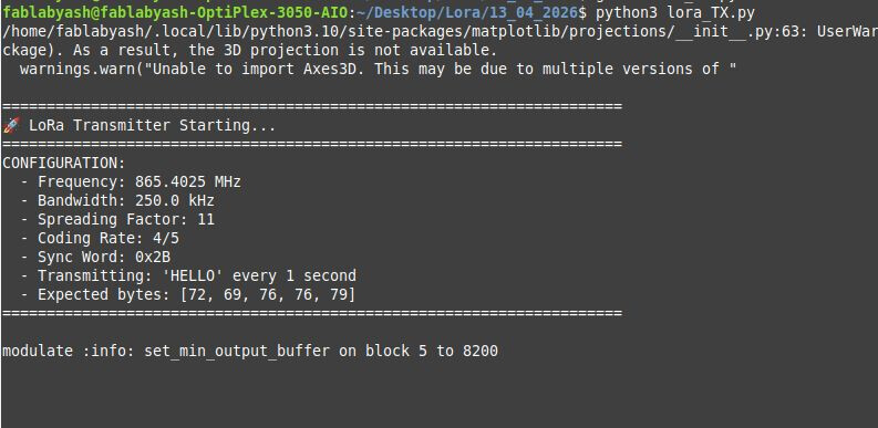
The terminal output confirms:
Frequency: 865.4025 MHz
Bandwidth: 250 kHz
Spreading Factor: 11
Coding Rate: 4/5
Sync Word: 0x2B
Transmitting: HELLO every 1 second
Expected bytes: [72, 69, 76, 76, 79]
This verifies the transmitter configuration before starting the receiver.
Part 9: The LoRa Receiver - Reversing the Process
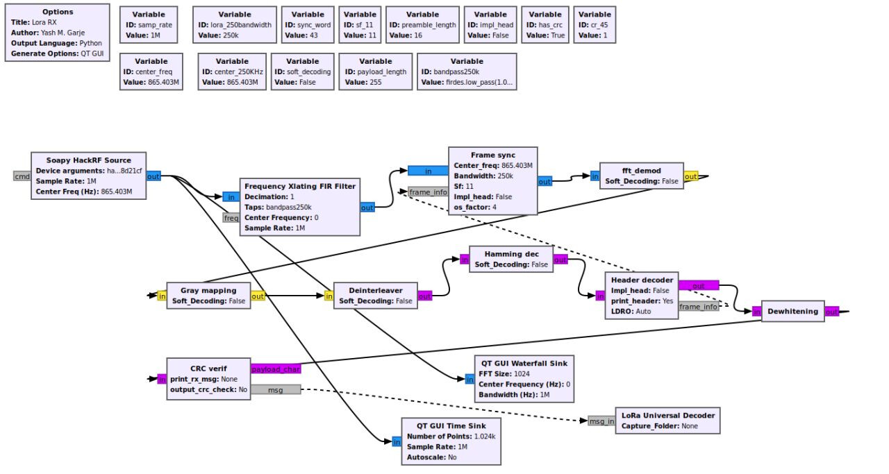
The receiver is the transmitter in reverse, but with added complexity for synchronization and error handling.
Block 1: HackRF Source
Captures RF signals at 865.4025 MHz and streams I/Q samples to GNU Radio.
Block 2: Preamble Detection
Purpose: Determine when a packet starts.
LoRa packets begin with 8 up-chirps (configurable, but often 8-16). The receiver continuously correlates incoming samples against a reference up-chirp.
When correlation peaks above a threshold → preamble detected → packet incoming.
Block 3: Synchronization
After preamble detection, the receiver locks onto:
- Symbol timing: Align processing windows with chirp boundaries
- Frequency offset: Measure and correct any carrier frequency error
This is critical. If symbol timing is off by even a few samples, the FFT will smear energy across multiple bins, and demodulation fails.
Block 4: FFT Demodulation
Purpose: Convert received chirps back into symbol numbers.
For each received chirp:
- Multiply by a reference down-chirp (dechirp)
- Apply FFT
- Find the peak bin → this is the symbol value
Why does this work?
When you multiply an up-chirp (increasing frequency) by a down-chirp (decreasing frequency), the result is a constant tone at a specific frequency determined by the starting point of the up-chirp.
The FFT converts this tone into a peak at a single frequency bin, directly revealing the transmitted symbol.
Block 5: Gray Demapping
Convert Gray-coded symbols back to binary bits.
Block 6: Deinterleaving
Reverse the interleaving process, grouping bits back into their original order.
Block 7: Hamming Decoding
Purpose: Detect and correct bit errors.
The decoder:
- Calculates parity checks
- Identifies error locations
- Corrects single-bit errors
- Outputs corrected data
If errors exceed the code’s correction capacity, the packet is flagged as corrupted.
Block 8: CRC Validation
Recalculate the CRC over the received payload and compare with the transmitted CRC.
- Match → packet valid
- Mismatch → packet corrupted, discard
Block 9: Dewhitening
XOR the data with the same pseudo-random sequence used in whitening to recover the original payload.
Block 10: Output
Convert bytes back to ASCII text and display.
Part 10: Receiver Signal Visualization
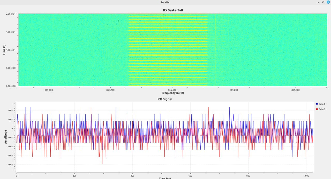
The waterfall display shows the received signal around 865 MHz. You can see the LoRa chirps arriving and being captured.
The time-domain plot shows the amplitude variation of the received signal. Notice the variations—these are the chirps, attenuated and distorted by propagation, but still decodable.
Part 11: The Breakthrough - Successful Reception
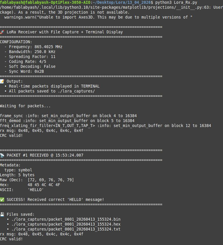
After weeks of debugging, the receiver terminal finally displayed:
Packet received:
Timestamp: 2024-XX-XX 12:34:56.789
Length: 5 bytes
Hex: 48 45 4C 4C 4F
ASCII: HELLO
CRC: Valid
Success.
The transmitted message was decoded correctly. The CRC validated. Data integrity confirmed.
What Fixed It?
The breakthrough came from fixing subtle issues in:
- CRC handling: The decoder was checking CRC before dewhitening, causing false rejections
- Byte reconstruction: Off-by-one errors in bit-to-byte conversion
- Packet boundary detection: Incorrect threshold for preamble correlation
Small bugs. Huge consequences.
Part 12: Continuous Operation
With the system working, I ran extended tests. The transmitter sent “HELLO” every second for hours. The receiver decoded consistently with zero packet loss (in a controlled lab environment with minimal interference).
This confirmed the system was stable, not just working by accident.
Part 13: Detailed Packet Analysis
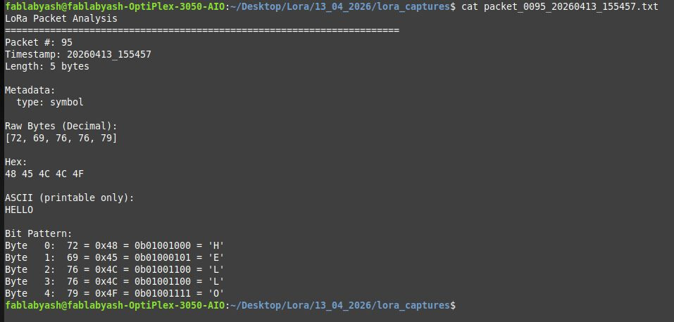
Each received packet was logged to a file for analysis:
Packet #42
Timestamp: 2024-XX-XX 12:34:56.789
Length: 5 bytes

Decimal:     72    69    76    76    79
Hexadecimal: 0x48  0x45  0x4C  0x4C  0x4F
Binary:      01001000 01000101 01001100 01001100 01001111
ASCII:       H     E     L     L     O

CRC: Valid
RSSI: -45 dBm
SNR: 12 dB
This level of detail was essential for debugging. I could:
- Verify byte-level data integrity
- Check ASCII conversion accuracy
- Monitor signal strength trends
- Detect patterns in packet loss (if any)
Part 14: Key Lessons Learned
Lesson 1: Transmitters vs. Receivers
Transmitters are straightforward because you control everything:
- You know the data format
- You generate the timing
- You set the frequency precisely
- You control modulation parameters
Receivers are hard because they must adapt to reality:
- Unknown timing offset
- Frequency drift
- Noise and interference
- Multipath fading
- Hardware imperfections
Building a robust receiver teaches you more about communication systems than anything else.
Lesson 2: Data Transformation Chains Are Error-Prone
Every format conversion is a potential bug:
Text → Bytes → Bits → Symbols → Chirps → RF
→ RF → Chirps → Symbols → Bits → Bytes → Text
A single off-by-one error anywhere destroys everything downstream.
Debug strategy:
- Instrument every stage
- Log intermediate outputs
- Verify data integrity at each step
- Work backwards from failures
Lesson 3: Synchronization Is The Hardest Part
You can have perfect demodulation logic, but if symbol timing is off by 10%, demodulation fails completely.
Synchronization requires:
- Preamble detection (coarse timing)
- Symbol boundary tracking (fine timing)
- Carrier frequency offset correction
- Clock drift compensation
Get this wrong, and nothing else matters.
Lesson 4: Error Correction Is Not Optional
Wireless channels are hostile. Noise, interference, and multipath fading corrupt bits constantly.
Without FEC (Forward Error Correction):
- Bit Error Rate (BER) might be 10^-3 (1 error per 1000 bits)
- A 100-byte packet has ~800 bits → 80% chance of at least one error
- Packet Error Rate (PER) = 80%
With FEC (Hamming codes, interleaving):
- Single-bit errors corrected automatically
- Burst errors spread across symbols and corrected
- PER drops to < 1%
Lesson 5: Debugging Requires Visibility
You can’t fix what you can’t see.
Essential debugging tools:
- Waterfall plots: Visualize signals in frequency domain
- Time-domain plots: Spot timing issues
- Constellation diagrams: Check modulation quality
- BER measurements: Quantify channel performance
- Packet logs: Track data integrity end-to-end
Add instrumentation early. It pays off.
Part 15: Understanding I/Q Samples (Deeper Dive)
Throughout this project, I mentioned “I/Q samples.” Let’s understand what these actually are.
The Problem: Representing Complex Signals
A radio wave is:
s(t) = A·cos(2πf·t + φ)
Where:
- A = amplitude
- f = frequency
- φ = phase
To digitally represent this, you need to capture both amplitude and phase. But a single number (like a regular audio sample) only captures amplitude.
The Solution: Quadrature Sampling
Represent the signal as two components:
- I (In-phase): Amplitude of the cos() component
- Q (Quadrature): Amplitude of the sin() component
Any signal can be written as:
s(t) = I(t)·cos(2πf·t) + Q(t)·sin(2πf·t)
Or, using complex notation:
s(t) = (I(t) + j·Q(t)) · e^(j2πft)
Why This Matters
With I/Q samples, you can:
- Measure instantaneous phase: φ = atan2(Q, I)
- Measure instantaneous amplitude: A = sqrt(I² + Q²)
- Shift frequency in software (just multiply by e^(j2πΔf·t))
- Implement any modulation/demodulation in software
This is why SDRs stream I/Q samples—they contain complete signal information.
Part 16: Why LoRa Works Where FSK Failed
Let’s revisit my early failures with FSK and understand why LoRa succeeded.
FSK Challenges
Narrow-band modulation:
- Energy concentrated at two frequencies
- Interference at either frequency destroys data
- Frequency offset directly causes errors
Binary symbols:
- Each symbol carries 1 bit
- Need high symbol rate for reasonable data rate
- High symbol rate = short symbol duration = harder synchronization
Noise sensitivity:
- SNR must be relatively high (~10 dB) for reliable decoding
LoRa Advantages
Spread spectrum:
- Energy spread across 250 kHz
- Narrow-band interference affects small portion of signal
- Processing gain: spreading then despreading improves SNR
Multi-bit symbols:
- Each symbol carries 11 bits (SF=11)
- Lower symbol rate for same data rate
- Long symbols (8 ms) make synchronization easier
Noise resilience:
- Can decode at negative SNR (signal weaker than noise)
- Chirps remain recognizable even in heavy interference
Doppler tolerance:
- Frequency offset shifts entire chirp uniformly
- FFT peak still identifiable, just at different bin
- Built-in frequency offset correction
This is why LoRa is used for long-range IoT applications—it works in harsh RF environments where simple modulation schemes fail.
Part 17: Real-World Considerations
Legal Compliance
Operating a transmitter requires regulatory compliance:
In India:
- 865-867 MHz is license-free for low-power devices
- Maximum EIRP: 1 W (30 dBm)
- Duty cycle limits may apply
- Outdoor operation may require additional permissions
Always check local regulations before transmitting.
Range Estimation
Theoretical LoRa range depends on:
Link budget calculation:
RX_power = TX_power + TX_gain - TX_loss - path_loss + RX_gain - RX_loss
For my setup:
- TX power: +10 dBm (HackRF output)
- TX antenna gain: +2 dBi
- Path loss (1 km, 865 MHz): ~97 dB
- RX antenna gain: +2 dBi
- RX sensitivity (SF=11): -136 dBm
RX_power = 10 + 2 - 0 - 97 + 2 - 0 = -83 dBm
This is well above sensitivity, suggesting ~1 km range is achievable.
In practice:
- Indoor walls: -10 to -20 dB additional loss
- Antenna placement: critical (elevation helps)
- Interference: unpredictable
- Multipath: causes fading
My lab tests (~10 meters) operated with ~40 dB link margin, essentially zero packet loss.
Part 18: What’s Next?
This project established a working baseline. Potential next steps:
1. Adaptive Data Rate (ADR)
Dynamically adjust SF based on link quality:
- Close range: SF=7 (faster data rate)
- Far range: SF=12 (longer range but slower)
Implement feedback mechanism where receiver reports SNR, and transmitter adjusts SF accordingly.
2. Bidirectional Communication
Current setup is simplex (one-way). Implement duplex:
- Time-division: transmit, then switch to receive
- Frequency-division: transmit and receive on different channels
- ACK/NACK protocol: confirm packet reception
3. Multi-Node Network
Expand to 3+ devices:
- Implement addressing (each device has unique ID)
- Media access control (prevent collisions)
- Routing (multi-hop communication)
4. Outdoor Range Testing
Characterize real-world performance:
- Open field: baseline range
- Urban: obstacle effects
- Elevated TX: ground-wave propagation
- Map coverage area
5. Interference Testing
Evaluate robustness:
- Co-channel interference (multiple LoRa transmitters)
- Adjacent-channel interference (other signals nearby)
- Impulsive noise (motors, switches)
6. Optimized Protocol
Replace GNU Radio with optimized C++ implementation:
- Lower latency
- Higher reliability
- Suitable for embedded deployment
Part 19: Resources and References
Hardware
- HackRF One: Great Scott Gadgets
- Antennas: 865 MHz quarter-wave (8.7 cm) or helical
- Cables: SMA-to-SMA, <1 meter to minimize loss
Software
- GNU Radio: gnuradio.org
- gr-lora: GitHub - rpp0/gr-lora
- Python 3.8+, PyQt5 for GUI
Learning Resources
- LoRa Modulation Basics: Semtech AN1200.22
- GNU Radio Tutorials: wiki.gnuradio.org/index.php/Tutorials
- DSP Guide: dspguide.com
Papers
- “LoRa Modulation Analysis” - investigate FFT-based demodulation
- “Chirp Spread Spectrum” - historical context and theory
Conclusion: What I Actually Learned
This project took months. Weeks of failures preceded the working system. But those failures taught me more than any textbook could.
Theoretical understanding is necessary but insufficient.
I knew FSK theory before starting. I understood phase modulation conceptually. But I didn’t truly understand wireless communication until I:
- Debugged timing recovery for hours
- Watched signals disappear into noise
- Fixed off-by-one errors in decoders
- Celebrated the first correctly decoded packet
Systems thinking matters.
Every block in the signal chain affects every other block. You can’t optimize the modulator without considering the demodulator. You can’t design error correction without understanding the channel.
Real implementations are messy.
Idealized textbooks show clean block diagrams and perfect waveforms. Reality involves:
- Clock drift
- Quantization noise
- Finite precision arithmetic
- Hardware bugs
- Unexpected interactions
Build, break, fix, repeat.
That’s how you learn. Not by reading—though that helps—but by building systems, watching them fail, understanding why, and fixing them.
If you want to understand wireless communication, don’t just read about it. Build a transmitter. Build a receiver. Send data. Watch it fail. Debug it. Make it work.
That’s when you’ll actually understand what’s happening when your phone connects to a cell tower.
Technical Specifications Summary
| Parameter | Value |
|---|---|
| Frequency | 865.4025 MHz |
| Bandwidth | 250 kHz |
| Modulation | LoRa (CSS) |
| Spreading Factor | 11 |
| Coding Rate | 4/5 |
| Sync Word | 0x2B |
| Preamble Length | 16 symbols |
| Sample Rate | 1 MSPS |
| Transmit Power | +10 dBm |
| Hardware | HackRF One (×2) |
| Software | GNU Radio 3.10, gr-lora |
| Operating System | Linux (Ubuntu 22.04) |
| Lab Distance | ~10 meters |
| Packet Loss | 0% (controlled environment) |
All experiments were conducted in a controlled laboratory environment using license-free frequency bands. Users must comply with local telecommunications regulations before operating radio transmitters. This article is for educational purposes only.